Hello and Welcome!
So in this blog post we’ll learn how to build a random forest classifier using scikit learn in python under 80 lines of python code.
NOTE:If you want to skip the explanation of snippets the fully working codes are available at the end of the blog along with the dataset.
The tools used are
Spyder IDE

Anaconda Distribution
First of all we need to import few dependencies that we’re going to work with
from pandas import Series, DataFrame
import pandas as pd
import numpy as np
import os
import matplotlib.pylab as plt
from sklearn.cross_validation import train_test_split
from sklearn.tree import DecisionTreeClassifier
from sklearn.metrics import classification_report
import sklearn.metrics
 # Feature Importance
from sklearn import datasets
from sklearn.ensemble import ExtraTreesClassifier
Now we need to tell our code to look for the directory where the dataset is located this is done by using the following
os.chdir("C:\TREES")
Now we need to read the csv file and drop not available values
AH_data = pd.read_csv("health.csv")
data_clean = AH_data.dropna()
Let’s describe the dataset now to see what we’re dealing with
BIO_SEX HISPANIC WHITE BLACK NAMERICAN \
count 4575.000000 4575.000000 4575.000000 4575.000000 4575.000000
mean 1.521093 0.111038 0.683279 0.236066 0.036284
std 0.499609 0.314214 0.465249 0.424709 0.187017
min 1.000000 0.000000 0.000000 0.000000 0.000000
25% 1.000000 0.000000 0.000000 0.000000 0.000000
50% 2.000000 0.000000 1.000000 0.000000 0.000000
75% 2.000000 0.000000 1.000000 0.000000 0.000000
max 2.000000 1.000000 1.000000 1.000000 1.000000

ASIAN age TREG1 ALCEVR1 ALCPROBS1 \
count 4575.000000 4575.000000 4575.000000 4575.000000 4575.000000
mean 0.040437 16.493052 0.176393 0.527432 0.369180
std 0.197004 1.552174 0.381196 0.499302 0.894947
min 0.000000 12.676712 0.000000 0.000000 0.000000
25% 0.000000 15.254795 0.000000 0.000000 0.000000
50% 0.000000 16.509589 0.000000 1.000000 0.000000
75% 0.000000 17.679452 0.000000 1.000000 0.000000
max 1.000000 21.512329 1.000000 1.000000 6.000000

ESTEEM1 VIOL1 PASSIST DEVIANT1 \
count ... 4575.000000 4575.000000 4575.000000 4575.000000
mean ... 40.952131 1.618579 0.102514 2.645027
std ... 5.381439 2.593230 0.303356 3.520554
min ... 18.000000 0.000000 0.000000 0.000000
25% ... 38.000000 0.000000 0.000000 0.000000
50% ... 40.000000 0.000000 0.000000 1.000000
75% ... 45.000000 2.000000 0.000000 4.000000
max ... 50.000000 19.000000 1.000000 27.000000

SCHCONN1 GPA1 EXPEL1 FAMCONCT PARACTV \
count 4575.000000 4575.000000 4575.000000 4575.000000 4575.000000
mean 28.360656 2.815647 0.040219 22.570557 6.290710
std 5.156385 0.770167 0.196493 2.614754 3.360219
min 6.000000 1.000000 0.000000 6.300000 0.000000
25% 25.000000 2.250000 0.000000 21.700000 4.000000
50% 29.000000 2.750000 0.000000 23.700000 6.000000
75% 32.000000 3.500000 0.000000 24.300000 9.000000
max 38.000000 4.000000 1.000000 25.000000 18.000000

PARPRES
count 4575.000000
mean 13.398033
std 2.085837
min 3.000000
25% 12.000000
50% 14.000000
75% 15.000000
max 15.000000
This is what we’re dealing with!
Now we set our predictors or our features and clean the target variables and devide the dataset into training and testing data (60:40 ratio)
Then we’re going to RandomForestClassifer from ensemble from sklearn
from sklearn.ensemble import RandomForestClassifier

Now finally let's build the forest

classifier=RandomForestClassifier(n_estimators=25)
classifier=classifier.fit(pred_train,tar_train)
Here 25 is the number of trees that the forest will contain.
Let’s printout the accuracy and confusion matrix
[[1428 92]
 [ 183 127]]
0.849726775956
89% Accuracy NOT BAD!! 😀
In the confusion matrix the diagonal indicates the number of true positive and true negative values and 92 and 183 tells about the false negative and false positive respectively
Time to display the importance of each attribute
# fit an Extra Trees model to the data
model = ExtraTreesClassifier()
model.fit(pred_train,tar_train)
# display the relative importance of each attribute
print(model.feature_importances_)

[ 0.02305763 0.01585706 0.01981318 0.01882172 0.00819704 0.00474358
 0.06132761 0.0596015 0.0433457 0.11824281 0.02111982 0.01668584
 0.03413818 0.05850854 0.05522334 0.044511 0.01733067 0.06630337
 0.05980527 0.07483757 0.01314004 0.06078445 0.05635996 0.0482441 ]
We see that whether the person has used marijuana has most importance and whether the person is Asian or not has least importance(LoL 🙂 )
Hold On we aren’t done yet,
Do we actually need 25 trees in our forest?
trees=range(25)
accuracy=np.zeros(25)

for idx in range(len(trees)):
 classifier=RandomForestClassifier(n_estimators=idx + 1)
 classifier=classifier.fit(pred_train,tar_train)
 predictions=classifier.predict(pred_test)
 accuracy[idx]=sklearn.metrics.accuracy_score(tar_test, predictions)

plt.cla()
plt.plot(trees, accuracy)
The above code determines the accuracy for trees upto range 25 and stores the accuracy of each of the result into an array and then plots it using plot function in python(No Graphwiz this time Thank God!)
Here’s the plot:
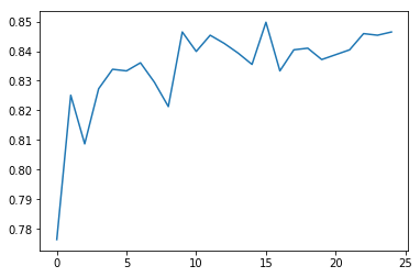
We see that when there was only one tree (just like a decision tree) the accuracy was just close to 83% and even with 25 trees the accuracy just increased upto 84%
CONCLUSION:
- Random forests do generalize well on the data
- Trees are themselves not interpreted and the entire forest is interpreted which can be a disadvantage as one tree may give the same result as 100 trees
The complete code:
# -*- coding: utf-8 -*-
"""
Created on Wed Nov 15 21:09:27 2017

@author: Aditya
"""

from pandas import Series, DataFrame
import pandas as pd
import numpy as np
import os
import matplotlib.pylab as plt
from sklearn.cross_validation import train_test_split
from sklearn.tree import DecisionTreeClassifier
from sklearn.metrics import classification_report
import sklearn.metrics
 # Feature Importance
from sklearn import datasets
from sklearn.ensemble import ExtraTreesClassifier

os.chdir("C:\TREES")

#Load the dataset

AH_data = pd.read_csv("health.csv")
data_clean = AH_data.dropna()

data_clean.dtypes
data_clean.describe()

#Split into training and testing sets

predictors = data_clean[['BIO_SEX','HISPANIC','WHITE','BLACK','NAMERICAN','ASIAN','age',
'ALCEVR1','ALCPROBS1','marever1','cocever1','inhever1','cigavail','DEP1','ESTEEM1','VIOL1',
'PASSIST','DEVIANT1','SCHCONN1','GPA1','EXPEL1','FAMCONCT','PARACTV','PARPRES']]

targets = data_clean.TREG1

pred_train, pred_test, tar_train, tar_test = train_test_split(predictors, targets, test_size=.4)

pred_train.shape
pred_test.shape
tar_train.shape
tar_test.shape

#Build model on training data
from sklearn.ensemble import RandomForestClassifier

classifier=RandomForestClassifier(n_estimators=25)
classifier=classifier.fit(pred_train,tar_train)

predictions=classifier.predict(pred_test)

print(sklearn.metrics.confusion_matrix(tar_test,predictions))
print(sklearn.metrics.accuracy_score(tar_test, predictions))


# fit an Extra Trees model to the data
model = ExtraTreesClassifier()
model.fit(pred_train,tar_train)
# display the relative importance of each attribute
print(model.feature_importances_)


"""
Running a different number of trees and see the effect
 of that on the accuracy of the prediction
"""

trees=range(25)
accuracy=np.zeros(25)

for idx in range(len(trees)):
 classifier=RandomForestClassifier(n_estimators=idx + 1)
 classifier=classifier.fit(pred_train,tar_train)
 predictions=classifier.predict(pred_test)
 accuracy[idx]=sklearn.metrics.accuracy_score(tar_test, predictions)

plt.cla()
plt.plot(trees, accuracy)
And the dataset used : [CLICK HERE]
I’ve blogged about the same analysis with decision trees here:Decision Tree Approach To Predict the Chances of A Person being Addicted to Substances or Alcohol
Feel Free to Comment or Contact me
